Author
Lucas Aragno
A couple of months ago I gave a talk at the NodeSummit about my experience using machine learning with JavaScript and a brief introduction to neural networks. In this post, I will focus on Neural Networks – reviewing additional examples of neural networks using synaptic, which is a library for neural networks for both NodeJS and the browser – before delving more into Machine Learning.
The Neuron
First, let’s do a quick recap of what a Neural Network is and how it is used. For this, we will start from the basic component of the neural network: The Neuron. This is a neuron. As you can see, a neuron has a set of inputs with its own weights plus a special input called a “Bias” which always has a value of 1. The goal of this structure is to establish that if all of the inputs of the neuron are 0, then the neuron will still have something after the activation function is applied.
Before moving onto activation function, we need to know how to compute the neuron state. We can accomplish this by adding every input multiplied by its weight, like so: L0 * W0 + L1 * W1 + […] + Ln * Wn + B * Wn+1
When we activate the neuron, it computes its state and runs the output through the Activation Function. The idea of the activation function is to “normalize” the result (usually between 0 and 1). The Activation Function is typically a Sigmoid Function:
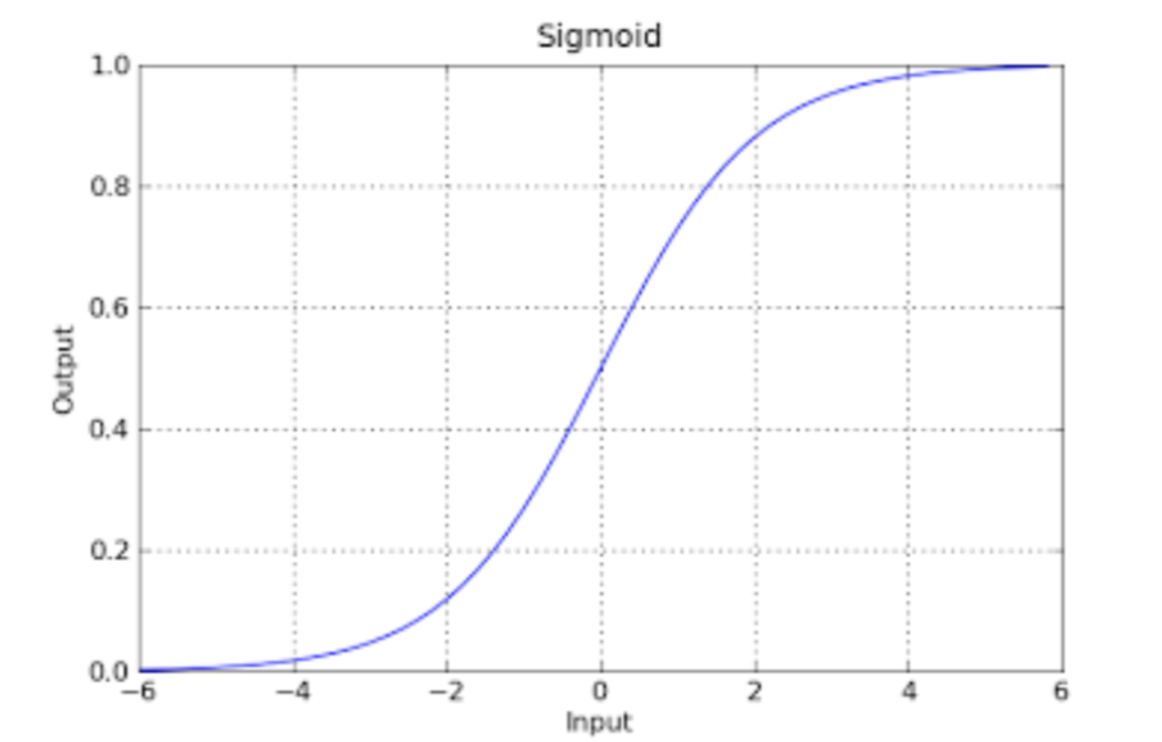
There are a variety of activation functions, including:
- Logistic Sigmoid
- Hyperbolic Tangent
- Hard Limit Functions
- Rectified Linear Unit
Here are additional resources to learn more about these activation functions: “Logistic Regression: Why Sigmoid Function?,” “Neural Networks 101,” and neural networking activation methods.
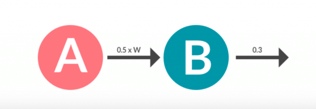
Neurons can perform beyond an activation function and can also project their output to another neuron:
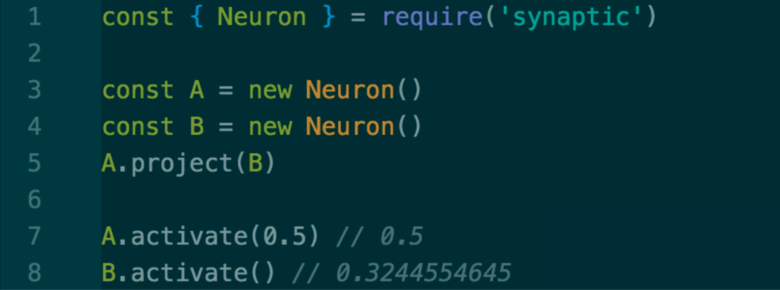
In this example, we are using the Neuron class from synaptic to create two networks: A and B. Then we project A to B: the output of A is going to act as the input of B. When we prompt A.activate(0.5), we are sending 0.5 as the output of the A neuron and it’s going to get multiplied by a weight (which will be random at first). It is then applied to an activation function on B to generate an output (0.3244554645) when B is activated.
It is important to note, as in the example, that if we call to activate with a value, that means we want that value to be the output of the neuron. If we call to activate without any value, it is going to perform the activation function with the neuron state.
Propagation
At this point, we have made a neural network composed of two neurons, but how does a network learn?
There is another operation that a neuron can perform: Propagation. When we propagate, we “adjust” the random weights using the error, in order to get a desired output based on an input and its error. From this, we can determine how far off from our desired output we were based on the output that we got for that input.
Sounds a little confusing, right? So let’s do an example:

Let’s train our little 2 neuron network so that whenever we get a 1 as the input, it will output a 0. For this example, let’s assume that an input of 1 represents “nice things” and an input of 0 represents “bad things.” On the other hand, an output of 0 represents “nice” and output of 1 represents “bad.” From there, it becomes a simple logical equation: If we input a 1, then we get an output of 0, therefore meaning to our network that “nice things are nice.”
Here we have the code. Lines 1 through 5 are basically what we did in our previous example: We create the A neuron and the B neuron and project A to B.
Then, we set a learning rate. This is one of our hyper-parameters that’s going to help us to reduce the “cost function” of the neural network by adjusting those weights to get the desired output. For now, this parameter may be kept as is and tweaked as you see fit, in order to achieve the desired results. (You can learn about the math behind that here.)
The next step is to loop the steps: A.activate, B.activate and B.propagate 20,000 times through a block of code that’s going to be our “training session:” To begin, activate A with 1, meaning that 1 x [randomWeight] is going to be the input of B. Then we activate B. Note that the first time this is done, you will likely get a higher number than 0 (perhaps even a 1), depending on the first randomWeight.
This is okay and it is why we propagate after the activation. Using the learning rate and the desired output for the previous input, it calculates the error from the previous activation and the 0 that we want to achieve. It then propagates that back to the connection between the neurons, adjusting the weights to get closer to the desired output: This is called backpropagation.
This will be done 20,000 times; adjusting and re-adjusting the weight 20,000 times, so that whenever we have a network input of, we get a 0 output. After the “training session,” if we activate A with a 1, then activating B should result in a number very close to 0. And voila!, our network just learn how to respond 0 whenever it gets a 1!
Neural Layers
Of course, this is just a basic example, because a real neural network is composed of many neurons adjusted in various layers.
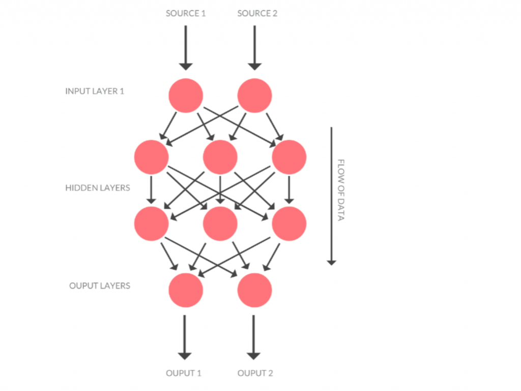
The first layer is called the Input Layer. This layer is comprised of the inputs provided by the engineer. The last layer is called the Output Layer, which will output the results of the activation of the network.
In between those two layers, there may be anywhere from zero to countless layers, which are called Hidden Layers. These layers can serve a variety of purposes, but their main objective is to get a better output on the neuron and number of Hidden Layers. The amount of neurons in Hidden Layers need to be tweaked depending on the case usage. You can learn more about Hidden Layers layers with “What’s Hidden in the Hidden Layers?” and “What does the hidden layer in a neural network compute?“
Building a Complex Network
Now that we’ve covered the basics of neural networks, let’s build a more complex network. This new network will be able to solve an XOR operation, wherein two inputs have one output. If you are unfamiliar with XOR, it looks like this:

To perform this function, we need to train our network to understand the XOR output of each set of inputs.
Before getting into code, let’s review our problem and define the amount of layers and neurons required. We will need:
- Our Input Layer, with 2 neurons (since we have 2 inputs)
- Our Output Layer, with 1 neuron (since our output is just 1 number)
- A Hidden Layer (to improve the results) with 2 neurons (since the rule of thumb is that the amount of neurons on the Hidden Layer is a number between the output and the input)

That’s how it would look on Synaptic. We can call directly the Layer and Network classes to create the layers with the amount of neurons that we want, then project the layers in the order that we need, creating the network with our layers in it. It would look something like this:

Now that we have our network, we can ‘train’ it by writing another ‘training session.’

As seen here, networks have the same API as the neurons’ input value we activate it with, propagating the error using the desired output to adjust its weights.
After all that training, we should be able to calculate the xorNet with values from the table and get the expected results. For example:
![]()
If you want to change the network results (for better or worse), you can adjust the learning rate and the number of loops per training session (hyper-parameters) to see what happens.
You might also want to try Synaptic counts with other classes, such as an Architect (to build different types of networks), a Trainer (to create those training sessions easily), and more utilities that could save you time. For more on these, I suggest reviewing the Synaptic Wiki.
This concludes the basics of Neural Networks with JavaScript. Stay tuned, as we will release another blog post to delve deeper into Machine Learning soon!